[LeetCode] Binary Indexed Tree, Fenwick Tree, BIT : 펜윅트리

 

Title	Solution	Acceptance	Difficulty
315	Count of Smaller Numbers After Self	42.60%	Hard
493	Reverse Pairs	26.60%	Hard
218	The Skyline Problem	36.10%	Hard
327	Count of Range Sum	35.90%	Hard
308	Range Sum Query 2D - Mutable	37.20%	Hard
307	Range Sum Query - Mutable	36.50%	Medium
1649	Create Sorted Array through Instructions	36.10%	Hard

 

315 Count of Smaller Numbers After Self

315. Count of Smaller Numbers After Self

Hard

3072100Add to ListShare

You are given an integer array nums and you have to return a new counts array. The counts array has the property where counts[i] is the number of smaller elements to the right of nums[i].

 

Example 1:

Input: nums = [5,2,6,1] Output: [2,1,1,0] Explanation: To the right of 5 there are 2 smaller elements (2 and 1). To the right of 2 there is only 1 smaller element (1). To the right of 6 there is 1 smaller element (1). To the right of 1 there is 0 smaller element.

 

 

 

 

493 Reverse Pairs

493. Reverse Pairs

Hard

1190134Add to ListShare

Given an array nums, we call (i, j) an important reverse pair if i < j and nums[i] > 2*nums[j].

You need to return the number of important reverse pairs in the given array.

Example1:

Input: [1,3,2,3,1] Output: 2

Example2:

Input: [2,4,3,5,1] Output: 3

Note:

1. The length of the given array will not exceed 50,000.
2. All the numbers in the input array are in the range of 32-bit integer.

Solution

---

Approach 1: Brute Force

Intuition

Do as directed in the question. We can simply check all the pairs if they are important reverse pairs or not.

Algorithm

• Iterate over ii from 00 to \text{size} - 1size−1
  • Iterate over jj from 00 to i - 1i−1
    • If \text{nums[j]} > 2 * \text{nums[i]}nums[j]>2∗nums[i], increment \text{count}count

Complexity Analysis

• Time complexity: O(n^2)O(n2)

  • We iterate over all the possible pairs wherein (i<ji<j) in the array which is O(n^2)O(n2)

• Space complexity: O(1)O(1) only constant extra space is required for nn, countcount etc.

Trivia

The above code can be expressed as one-liner in Python:

Herein, we iterate over all the pairs and store the boolean values for \text{nums[i]}>2*\text{nums[j]}nums[i]>2∗nums[j]. Finally, we count the number of \text{true}true in the array and return the result.

---

Approach 2: Binary Search Tree

Intuition

In Approach 1, for each element ii, we searched the subarray [0,i)[0,i) for elements such that their value is greater than 2*\text{nums[i]}2∗nums[i]. In the previous approach, the search is linear. However, we need to make the process efficient. Maybe, memoization can help, but since, we need to compare the elements, we cannot find a linear DP solution.

Observe that the indices of the elements in subarray [0,i)[0,i) don't matter as we only require the count. So, we can sort the elements and perform binary search on the subarray. But, since the subarray keeps growing as we iterate to the next element, we need a data structure to store the previous result as well as to allow efficient searching(preferably O(\log n)O(logn)) - Binary Search Tree(BST) could be a good bet.

Refreshing BST

BST is a rooted binary tree, wherein each node is associated with a value and has 2 distinguishable sub-trees namely leftleft and rightright subtree. The left subtree contains only the nodes with lower values than the parent's value, while the right subtree conatins only the nodes with greater values than the parent's value.

Voila!

This is exactly what is required. So, if we store our elements in BST, then we can search the larger elements thus eliminating the search on smaller elements altogether.

Algorithm

Define the \text{Node}Node of BST that stores the \text{val}val and pointers to the \text{left}left and \text{right}right. We also need a count of elements(say \text{count\_ge}count_ge) in the subtree rooted at the current node that are greater than or equal to the current node's \text{val}val. \text{count\_ge}count_ge is initialized to 1 for each node and \text{left}left, \text{right}right pointers are set to \text{NULL}NULL.

We define the \text{insert}insert routine that recursively adds the given \text{val}val as an appropriate leaf node based on comparisons with the Node.valNode.val. Each time, the given valval is smaller than Node.valNode.val, we increment the \text{count\_ge}count_ge and move the valval to the right subtree. While, if the valval is equal to the current NodeNode, we simply increment the \text{count\_ge}count_ge and exit. While, we move to the left subtree in case (\text{val}<\text{Node.val})(val<Node.val).

We also require the searchsearch routine that gives the count of number of elements greater than or equal to the \text{target}target. In the \text{search}search routine, if the headhead is NULL, return 0. Otherwise, if \text{target}==\text{head.val}target==head.val, we know the count of values greater than or equal to the \text{target}target, hence simply return \text{head.count\_ge}head.count_ge. In case, \text{target}<\text{head.val}target<head.val, the ans is calculated by adding \text{Node.count\_ge}Node.count_ge and recursively calling the \text{search}search routine with \text{head.left}head.left. And if \text{target}>\text{head.val}target>head.val, ans is obtained by recursively calling the \text{search}search routine with \text{head.right}head.right.

Now, we can get to our main logic:

• Iterate over ii from 00 to (size-1)(size−1) of \text{nums}nums :
  • Search the existing BST for \text{nums[i]} * 2 + 1nums[i]∗2+1 and add the result to \text{count}count
  • Insert \text{nums[i]}nums[i] to the BST, hence updating the \text{count\_ge}count_ge of the previous nodes

 

 

1 / 15

Complexity analysis

• Time complexity: O(n^2)O(n2)
  • The best case complexity for BST is O(\log n)O(logn) for search as well as insertion, wherein, the tree formed is complete binary tree
  • Whereas, in case like [1,2,3,4,5,6,7,8,...], insertion as well as search for an element becomes O(n)O(n) in time, since, the tree is skewed in only one direction, and hence, is no better than the array
  • So, in worst case, for searching and insertion over n items, the complexity is O(n*n)O(n∗n)
• Space complexity: O(n)O(n) extra space for storing the BST in \text{Node}Node class.
  
  

---

Approach 3: BIT

Intuition

The problem with BST is that the tree can be skewed hence, making it O(n^2)O(n2) in complexity. So, need a data structure that remains balanced. We could either use a Red-black or AVL tree to make a balanced BST, but the implementation would be an overkill for the solution. We can use BIT (Binary Indexed Tree, also called Fenwick Tree) to ensure that the complexity is O(n\log n)O(nlogn) with only 12-15 lines of code.

BIT Overview:

Fenwick Tree or BIT provides a way to represent an array of numbers in an array(can be visualized as tree), allowing prefix/suffix sums to be calculated efficiently(O(\log n)O(logn)). BIT allows to update an element in O(\log n)O(logn) time.

We recommend having a look at BIT from the following link before getting into details:

• https://www.topcoder.com/community/data-science/data-science-tutorials/binary-indexed-trees/

So, BIT is very useful to accumulate information from front/back and hence, we can use it in the same way we used BST to get the count of elements that are greater than or equal to 2 * \text{nums[i]} + 12∗nums[i]+1 in the existing tree and then adding the current element to the tree.

Algorithm

First, lets review the BIT \text{query}query and \text{update}update routines of BIT. According to the convention, \text{query}query routine goes from \text{index}index to 00, i.e., \text{BIT[i]}BIT[i] gives the sum for the range [0,index][0,index], and \text{update}update updates the values from current \text{index}index to the end of array. But, since, we require to find the numbers greater than the given index, as and when we update an index, we update all the ancestors of the node in the tree, and for \text{search}search, we go from the node to the end.

The modified \text{update}update algorithm is:

update(BIT, index, val): while(index > 0): BIT[index] += val index -= (index & (-index))

Herein, we find get the next index using: \text{index -= index \& (-index)}index -= index & (-index), which is essentially subtracting the rightmost 1 from the \text{index}index binary representation. We update the previous indices since, if an element is greater than the index

And the modified \text{query}query algorithm is:

query(BIT,index): sum=0 while(index<BIT.size): sum+=BIT[index] index+=(index&(-index))

Herein, we find get the next index using: \text{index += index \& (-index)}index += index & (-index). This gives the suffix sum from indexindex to the end.

So, the main idea is to count the number of elements greater than 2*\text{nums[i]}2∗nums[i] in range [0,i)[0,i) as we iterate from 00 to \text{size-1}size-1. The steps are as follows:

• Create a copy of \text{nums}nums, say \text{nums\_copy}nums_copy ans sort \text{nums\_copy}nums_copy. This array is actually used for creating the Binary indexed tree
• Initialize \text{count}=0count=0 and \text{BIT}BIT array of size \text{size(nums)} + 1size(nums)+1 to store the BIT
• Iterate over ii from 00 to \text{size(nums)}-1size(nums)−1 :
  • Search the index of element not less than 2*\text{nums[i]}+12∗nums[i]+1 in \text{nums\_copy}nums_copy array. \text{query}query the obtained index+1 in the \text{BIT}BIT, and add the result to \text{count}count
  • Search for the index of element not less than nums[i]nums[i] in \text{nums\_copy}nums_copy. We need to \text{update}update the BIT for this index by 1. This essentially means that 1 is added to this index(or number of elements greater than this index is incremented). The effect of adding 11 to the index is passed to the ancestors as shown in \text{update}update algorithm

Complexity analysis

• Time complexity: O(n\log n)O(nlogn)
  • In \text{query}query and \text{update}update operations, we see that the loop iterates at most the number of bits in \text{index}index which can be at most nn. Hence, the complexity of both the operations is O(\log n)O(logn)(Number of bits in nn is \log nlogn)
  • The in-built operation \text{lower\_bound}lower_bound is binary search hence O(\log n)O(logn)
  • We perform the operations for nn elements, hence the total complexity is O(n\log n)O(nlogn)
• Space complexity: O(n)O(n). Additional space for \text{BITS}BITS array
  
  

---

Approach 4: Modified Merge Sort

Intuition

In BIT and BST, we iterate over the array, dividing the array into 3 sections: already visited and hence added to the tree, current node and section to be visited. Another approach could be divide the problem into smaller subproblems, solving them and combining these problems to get the final result - Divide and conquer. We see that the problem has a great resemblance to the merge sort routine. The question is to find the inversions such that \text{nums[i]}>2 * \text{nums[j]}nums[i]>2∗nums[j] and i<ji<j. So, we can easily modify the merge sort to count the inversions as required.

Mergesort

Mergesort is a divide-and-conquer based sorting technique that operates in O(n\log n)O(nlogn) time. The basic idea to divide the array into several sub-arrays until each sub-array is single element long and merging these sublists recursively that results in the final sorted array.

Algorithm

We define \text{mergesort\_and\_count}mergesort_and_count routine that takes parameters an array say AA and \text{start}start and \text{end}end indices:

• If \text{start}start>=\text{end}end this implies that elements can no longer be broken further and hence we return 0
• Otherwise, set \text{mid}=(\text{start} + \text{end})/2mid=(start+end)/2
• Store countcount by recursively calling \text{mergesort\_and\_count}mergesort_and_count on range \text{[start,mid]}[start,mid] and \text{[mid+1,end]}[mid+1,end] and adding the results. This is the divide step on our routine, breaking it into the 2 ranges, and finding the results for each range separately
• Now, we that we have separately calculated the results for ranges \text{[start,mid]}[start,mid] and \text{[mid+1,end]}[mid+1,end], but we still have to count the elements in \text{[start,mid]}[start,mid] that are greater than 2 * elements in \text{[mid+1,end]}[mid+1,end]. Count all such elements and add the result to \text{count}count
• Finally, \text{merge}merge the array from \text{start}start to \text{end}end
  • Make 2 array : LL from elements in range \text{[start,mid]}[start,mid] and RR from elements in range \text{R[mid+1,end]}R[mid+1,end]
  • Keep pointers ii and jj to LL and RR respectively both initialized to start to the arrays
  • Iterate over kk from \text{start}start to \text{end}end and set \text{A[k]}A[k] to the smaller of \text{L[i]}L[i] or \text{R[j]}R[j] and increment the respective index

Complexity analysis

• Time complexity: O(n\log n)O(nlogn)

  • In each step we divide the array into 2 sub-arrays, and hence, the maximum times we need to divide is equal to O(\log n)O(logn)
  • Additional O(n)O(n) work needs to be done to count the inversions and to merge the 2 sub-arrays after sorting. Hence total time complexity is O(n\log n)O(nlogn)

• Space complexity: O(n)O(n). Additional space for storing LL and RR arrays

---

Shoutout to @FUN4LEETCODE for the brilliant post!

 

 

 

 

 

 

218 The Skyline Problem

218. The Skyline Problem

Hard

2635149Add to ListShare

A city's skyline is the outer contour of the silhouette formed by all the buildings in that city when viewed from a distance. Given the locations and heights of all the buildings, return the skyline formed by these buildings collectively.

The geometric information of each building is given in the array buildings where buildings[i] = [lefti, righti, heighti]:

• lefti is the x coordinate of the left edge of the ith building.
• righti is the x coordinate of the right edge of the ith building.
• heighti is the height of the ith building.

You may assume all buildings are perfect rectangles grounded on an absolutely flat surface at height 0.

The skyline should be represented as a list of "key points" sorted by their x-coordinate in the form [[x1,y1],[x2,y2],...]. Each key point is the left endpoint of some horizontal segment in the skyline except the last point in the list, which always has a y-coordinate 0 and is used to mark the skyline's termination where the rightmost building ends. Any ground between the leftmost and rightmost buildings should be part of the skyline's contour.

Note: There must be no consecutive horizontal lines of equal height in the output skyline. For instance, [...,[2 3],[4 5],[7 5],[11 5],[12 7],...] is not acceptable; the three lines of height 5 should be merged into one in the final output as such: [...,[2 3],[4 5],[12 7],...]

 

Example 1:

Input: buildings = [[2,9,10],[3,7,15],[5,12,12],[15,20,10],[19,24,8]] Output: [[2,10],[3,15],[7,12],[12,0],[15,10],[20,8],[24,0]] Explanation: Figure A shows the buildings of the input. Figure B shows the skyline formed by those buildings. The red points in figure B represent the key points in the output list.

Example 2:

Input: buildings = [[0,2,3],[2,5,3]] Output: [[0,3],[5,0]]

 

Constraints:

• 1 <= buildings.length <= 104
• 0 <= lefti < righti <= 231 - 1
• 1 <= heighti <= 231 - 1
• buildings is sorted by lefti in non-decreasing order.

Solution

---

Approach 1: Divide and Conquer

Solution Template

The problem is a classical example of divide and conquer approach, and typically implemented exactly the same way as merge sort algorithm.

Let's follow here a solution template for divide and conquer problems :

• Define the base case(s).

• Split the problem into subproblems and solve them recursively.

• Merge the subproblems solutions into the problem solution.

Algorithm

getSkyline for n buildings :

• If n == 0 : return an empty list.

• If n == 1 : return the skyline for one building (it's straightforward).

• leftSkyline = getSkyline for the first n/2 buildings.

• rightSkyline = getSkyline for the last n/2 buildings.

• Merge leftSkyline and rightSkyline.

Now let's discuss each step in more details.

Base Cases

The first base case is an empty buildings list. Then the skyline is an empty list, too.

The second base case is the only one building in the list, when the skyline construction is quite straightforward.

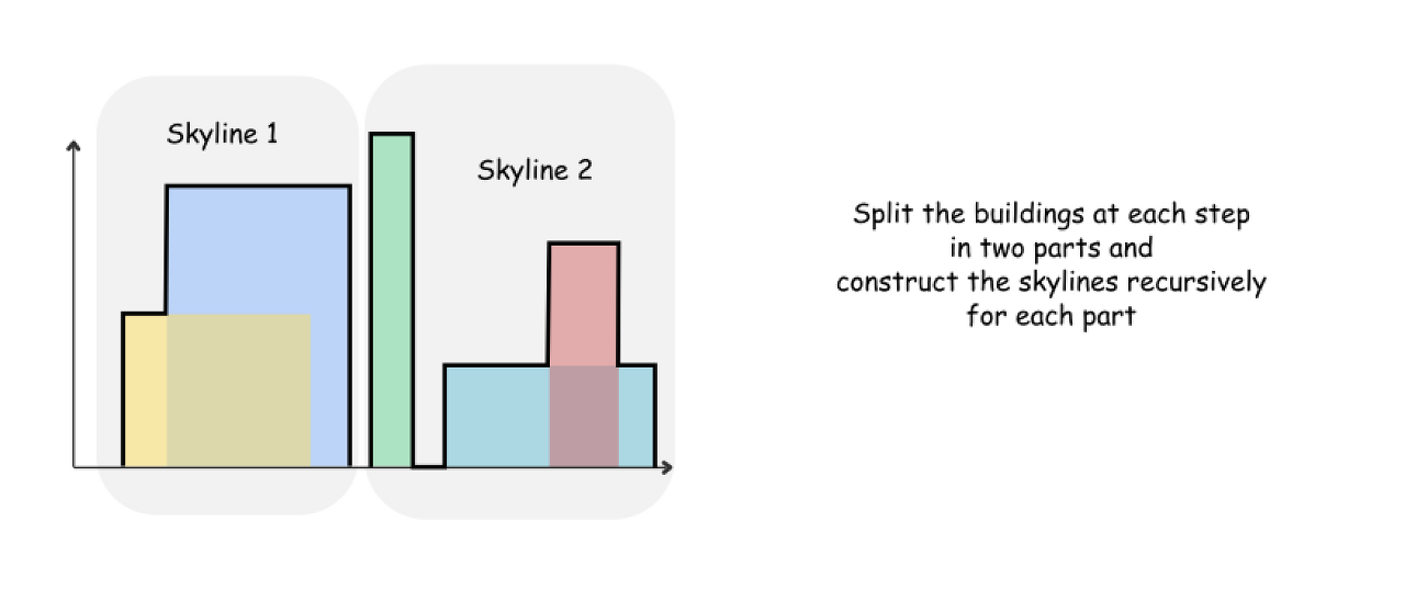
How to split the problem

The idea is the same as for merge sort : at each step split the list exactly in two parts : from 0 to n/2 and from n/2 to n, and then construct the skylines recursively for each part.

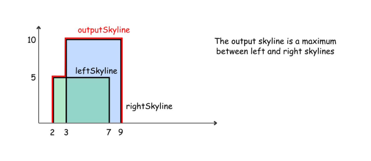
How to merge two skylines

The algorithm for merge function is quite straightforward and based on the same merge sort logic : the height of an output skyline is always a maximum between the left and right skylines.

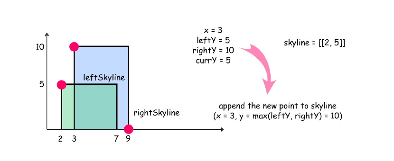
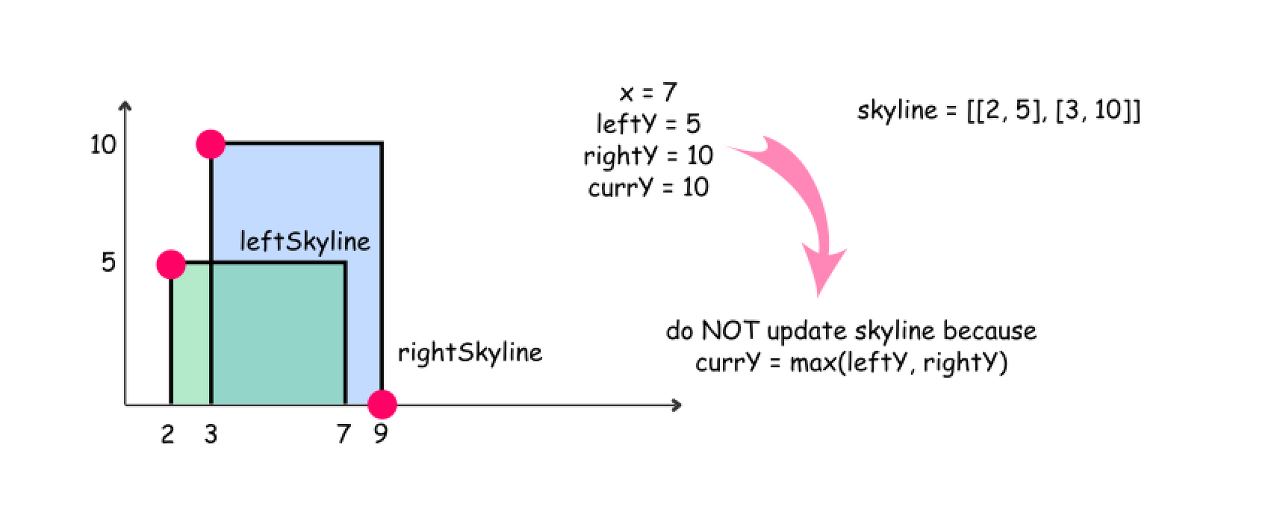
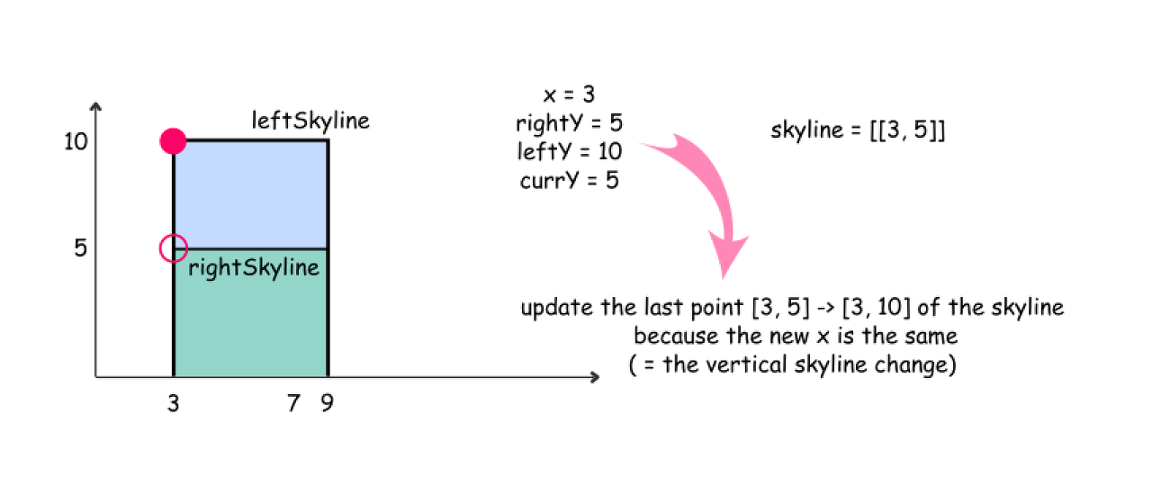
Let's use here two pointers pR and pL to track the current element index in both skylines, and three integers leftY, rightY, and currY to track the current height for the left skyline, right skyline and the merged skyline.

mergeSkylines (left, right) :

• currY = leftY = rightY = 0

• While we're in the region where both skylines are present (pR < nR and pL < nL) :

  • Pick up the element with the smallest x coordinate. If it's an element from the left skyline, move pL and update leftY. If it's an element from the right skyline, move pR and update rightY.

  • Compute the largest height at the current point : maxY = max(leftY, rightY).

  • Update an output skyline by (x, maxY) point, if maxY is not equal to currY.

• While there are still elements in the left skyline (pL < nL), process them following the same logic as above.

• While there are still elements in the right skyline (pR < nR), process them following the same logic as above.

• Return output skyline.

Here are three usecases to illustrate the merge algorithm execution

Implementation

• Time complexity : \mathcal{O}(N \log N)O(NlogN), where NN is number of buildings. The problem is an example of Master Theorem case II : T(N) = 2 T(\frac{N}{2}) + 2NT(N)=2T(2N​)+2N, that results in \mathcal{O}(N \log N)O(NlogN) time complexity.

• Space complexity : \mathcal{O}(N)O(N).

  • We use the output variable to keep track of the results.

 

 

 

 

 

 

 

 

 

 

327 Count of Range Sum

327. Count of Range Sum

Hard

954108Add to ListShare

Given an integer array nums, return the number of range sums that lie in [lower, upper] inclusive.
Range sum S(i, j) is defined as the sum of the elements in nums between indices i and j (i ≤ j), inclusive.

Note:
A naive algorithm of O(n2) is trivial. You MUST do better than that.

Example:

Input: nums = [-2,5,-1], lower = -2, upper = 2, Output: 3 Explanation: The three ranges are : [0,0], [2,2], [0,2] and their respective sums are: -2, -1, 2.

 

Constraints:

• 0 <= nums.length <= 10^4

 

 

 

308 Range Sum Query 2D - Mutable

구글

308. Range Sum Query 2D - Mutable

Hard

47561Add to ListShare

Given a 2D matrix matrix, find the sum of the elements inside the rectangle defined by its upper left corner (row1, col1) and lower right corner (row2, col2).

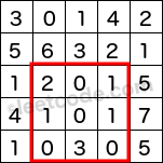
The above rectangle (with the red border) is defined by (row1, col1) = (2, 1) and (row2, col2) = (4, 3), which contains sum = 8.

Example:

Given matrix = [ [3, 0, 1, 4, 2], [5, 6, 3, 2, 1], [1, 2, 0, 1, 5], [4, 1, 0, 1, 7], [1, 0, 3, 0, 5] ] sumRegion(2, 1, 4, 3) -> 8 update(3, 2, 2) sumRegion(2, 1, 4, 3) -> 10

Note:

1. The matrix is only modifiable by the update function.
2. You may assume the number of calls to update and sumRegion function is distributed evenly.
3. You may assume that row1 ≤ row2 and col1 ≤ col2.

Solution

---

Approach 1: Brute Force

We use the same brute force method as we used in 2D Immutable version to calculate the sum of region. In addition to the previous problem, here we have to update the value of the matrix as well, which we simply do with data[row][col] = val.

Algorithm

Below is the implementation of this approach.

Complexity Analysis

• Time Complexity

  • sumRegion - O(MN)O(MN) per query. Where MM and NN represents the number of rows and columns respectively, each sumRegion query can go through at most M \times NM×N elements.

  • update - O(1)O(1) per query.

• Space Complexity: O(1)O(1).

---

Approach 2: Using Binary Indexed Tree

Intuition

The problem differs than the 2D Immutable version as there is an additional update method that changes the values present inside the matrix, hence it's not even a good choice to cache or pre-compute all the results. There is a special data structure called Binary Indexed Tree that we will use to solve this problem efficiently which is based on the idea of storing the partial sums. We then use these partial sums to obtain the overall sum in the sumRegion method. The way we store these partial sums in a Binary Indexed Tree (BIT), a.k.a. Fenwick Tree, allows us to achieve both the update and query to be done in logarithmic time.

Consider the case of 1-D array. Assume we have an array nums of size 8 (nums[1], nums[2] ... nums[8]) (1-based indexing). We store the partial sums of the array nums in another array bit of size 8 (bit[1], bit[2] ... bit[8]). The idea is to compute each value of bit array in a way that allows us to "quickly" compute the sum as well as update the values for the array nums. We do it using the idea of bit manipulation.

Each number can be represented as sum of power of two's and this is what will allow us to obtain the overall sum from the partial sums. For example, 7 can be represented as 1 + 2 + 4 = (2^{0} + 2^{1} + 2^{2})1+2+4=(20+21+22) hence whenever we want to calculate the cumulative sum till 7th index in the nums array, we will utilize the values stored in the 1st, 2nd and 4th index in the bit array. Here in case of Binary Indexed Tree, the 1st, 2nd and 4th index of the bit array will store the non-overlapping partial sums which can be added up to obtain the cumulative sum till 7th index in the nums array. Hence, we have cum\_sum(7) = bit[1] + bit[2] + bit[4] = a[1] + a[2] + ... + a[7]cum_sum(7)=bit[1]+bit[2]+bit[4]=a[1]+a[2]+...+a[7] (where cum_sum(7) refers to cumulative sum till 7th index of nums array). But how do we obtain the sum in such a manner? For this, consider the bit array as shown below (let's assume that we can efficiently obtain the below mentioned array, we'll discuss later how we can actually do it).

bit[1] = nums[1] bit[2] = nums[1] + nums[2] bit[3] = nums[3] bit[4] = nums[1] + nums[2] + nums[3] + nums[4] bit[5] = nums[5] bit[6] = nums[5] + nums[6] bit[7] = nums[7] bit[8] = nums[1] + nums[2] + nums[3] + nums[4] + nums[5] + nums[6] + nums[7] + nums[8]

When we try to calculate cumulative sum till any index n the steps that we follow are.

1. Decompose n as the sum of power of 2's. Let's say n = n_{1} + n_{2} + ... + n_{k}n=n1​+n2​+...+nk​ where each of the number n_{i}ni​ is a number which is a power of 2. For example, When n = 7n=7, we have n_{1} = 1, n_{2} = 2, n_{3} = 4 (7 = 1 + 2 + 4)n1​=1,n2​=2,n3​=4(7=1+2+4)

2. The cumulative sum till index n in the nums array can then be obtained with the help of bit array as cum\_sum(n) = bit[n_{1}] + bit[n_{2}] + ... + bit[n_{k}]cum_sum(n)=bit[n1​]+bit[n2​]+...+bit[nk​]

As mentioned before, since we'll store the values in the bit array as non-overlapping partial sums, that's why step 2 is possible and gives us the cumulative sum as the sum of the values from the bit array. The question that we must ask now is - How can we build the bit array in such a manner? For this, we need to do two things.

1. Understand lsb (least significant bit, non-zero) of a number.

2. Observe the pattern of occurence of each number from nums array in the bit array.

LSB (least significant bit)

Consider the binary representation of 5 (5 -> 101). The least significant (non-zero) bit of a number is obtained by taking the right most non-zero bit from the binary representation and ignoring all the other bits (i.e. considering all the other bits as 0). Hence lsb(5) = 001 (considering only the rightmost non-zero bit and ignoring all others). Similarly lsb(6) = 010. Why? Since 6 -> 110 and the right most set bit occurs at the second position.

Next, let's notice the occurence of each element of nums array in the bit array as follows.

nums[1] isPresentIn -> bit[1], bit[2], bit[4], bit[8] nums[2] isPresentIn -> bit[2], bit[4], bit[8] nums[3] isPresentIn -> bit[3], bit[4], bit[8] nums[4] isPresentIn -> bit[4], bit[8] nums[5] isPresentIn -> bit[5], bit[6], bit[8] nums[6] isPresentIn -> bit[6], bit[8] nums[7] isPresentIn -> bit[7], bit[8] nums[8] isPresentIn -> bit[8]

Let's convert all the indices shown above into their binary representation. We then have (indices for nums array on the LHS and bit array on the RHS)

LHS -> RHS nums[0001] -> bit[0001], bit[0010], bit[0100], bit[1000] nums[0010] -> bit[0010], bit[0100], bit[1000] nums[0011] -> bit[0011], bit[0100], bit[1000] nums[0100] -> bit[0100], bit[1000], nums[0101] -> bit[0101], bit[0110], bit[1000] nums[0110] -> bit[0110], bit[1000] nums[0111] -> bit[0111], bit[1000] nums[1000] -> bit[1000]

On seeing the pattern above, we can notice that the sequence of indices on the RHS can be obtained by continuously adding the number to it's lsb, starting from the index on the LHS.

Example

0101 -> (add 0001) -> 0110 -> (add 0010) -> 1000

We can use this observation to build the bit array as we now know all the indices in the bit array where a particular value from the nums array occurs.

Note: We have used 1-based indexing at all the places in the 1-D BIT explanation part.

The process of adding a particular number val to the appropriate locations in the bit array is what is known as the update process in a Binary Indexed Tree. Hence we can re-write the above code as.

Below is the animation of the buildBIT process for the array [2, 3, 1, 2, 4, 1, 2, 3]. We initialize all the elements of the bit array to zero and then build it.

 

Having a separate update method also allows us to perform the "updates" in a Binary Indexed Tree, i.e. if we want to change the values of nums[i] from an old value a to new updated value b, we simply calculate the difference b - a and call the update function as updateBIT(i, b - a) (note that we do not change the actual nums array, only the bit array changes). We still haven't implemented the sumRegion for our 1-D example here. This is known as "query" method for a Binary Indexed Tree. When query method is called for a particular index i on the Binary Indexed Tree, it returns the cumulative sum till the index i. Similar to update method, where we kept adding the lsb of the index to itself, here, we'll keep subtracting the lsb of the index from itself to calculate the cumulative sum from partial sums stored in bit array. The code is as follows.

Below is the animation of the query process for the array [2, 3, 1, 2, 4, 1, 2, 3] in case of index = 7, i.e. we are trying to calculate the cumulative sum till the 7th index of the nums array.

 

We can now use the queryBIT and updateBIT methods to obtain the sum between any two indices (i, j) and can update the value at any given index i as follows

Complexity Analysis

• Time Complexity

  • Update (1D) - O(\log{N})O(logN)

  • Query (1D) - O(\log{N})O(logN)

  • Build (1D) - O(N \cdot \log{N})O(N⋅logN)

  • Here N denotes the number of elements present in the array. Maximum number of steps that we'll have to iterate for update and query method is upper bounded by the number of bits in the binary representation of the size of the array (N).

• Space Complexity

  • O(N)O(N) - Since we'll need an extra bit array to store the non-overlapping partial sums.

We now have the required pre-requisites to implement an efficient solution for the case of 2D arrays (or matrix), which we'll see next.

Note: The build method can be optimized further and can be done in time O(N)O(N). We do this by adding the entry from the nums array to the immediate next entry in the bit array, i.e. the next higher index that the value from the nums array contributes to. Below is the implementation for this

2D BIT

Till now, we have seen how to perform "query" and "update" in case of 1-D example. We'll try to extend this to 2D array (matrix) now.

In case of 1D example, we were iterating directly over the indices of the array in 1 direction, but here in the case of a matrix, we have a 2-dimensional indices. Hence in order to use the concept of BIT for 2D case, we'll iterate in both the directions, i.e. over the rows and columns of the matrix to perform the update and query method. If i and j represents the indices corresponding to rows and columns that are used for iterating over the matrix, we simply increment these variables by lsb(i) and lsb(j) in the update operation and decrement by lsb(i) and lsb(j) in decrement operation. Another change that happens in the case of 2D bit is, the partial sums that we store now are corresponding to partial sum of the non-overlapping sub-rectangles or sub-matrix present in the matrix.

The update and the query for the 2D matrix then are as follows.

The build method in case of 2D array can be implemented as follows.

We can now use the queryBIT and updateBIT methods to obtain the sum for any rectangular region, denoted by (row1, col1) and (row2, col2) and can update the value at any given location (row, col) as follows

The overall solution code for 2D case is as follows.

Note that there will be some minor modifications in the final implementation from the code snippets provided above as the input that we have here is based on 0-based indexing and not 1-based indexing. Hence we'll take that into account in the final implementation.

Complexity Analysis

• Time Complexity

  • Update (2D) - O(\log{N} \cdot \log{M})O(logN⋅logM)

  • Query (2D) - O(\log{N} \cdot \log{M})O(logN⋅logM)

  • Build (2D) - O(N \cdot M \cdot \log{N} \cdot \log{M})O(N⋅M⋅logN⋅logM)

  • Here N denotes the number of rows and M denotes the number of columns.

• Space Complexity

  • O(NM)O(NM) - Since we'll need an extra bit matrix to store the non-overlapping partial sums

 

 

307 Range Sum Query - Mutable

페이스북

 

307. Range Sum Query - Mutable

Medium

166098Add to ListShare

Given an array nums and two types of queries where you should update the value of an index in the array, and retrieve the sum of a range in the array.

Implement the NumArray class:

• NumArray(int[] nums) Initializes the object with the integer array nums.
• void update(int index, int val) Updates the value of nums[index] to be val.
• int sumRange(int left, int right) Returns the sum of the subarray nums[left, right] (i.e., nums[left] + nums[left + 1], ..., nums[right]).

 

Example 1:

Input ["NumArray", "sumRange", "update", "sumRange"] [[[1, 3, 5]], [0, 2], [1, 2], [0, 2]] Output [null, 9, null, 8] Explanation NumArray numArray = new NumArray([1, 3, 5]); numArray.sumRange(0, 2); // return 9 = sum([1,3,5]) numArray.update(1, 2); // nums = [1,2,5] numArray.sumRange(0, 2); // return 8 = sum([1,2,5])

 

Constraints:

• 1 <= nums.length <= 3 * 104
• -100 <= nums[i] <= 100
• 0 <= index < nums.length
• -100 <= val <= 100
• 0 <= left <= right < nums.length
• At most 3 * 104 calls will be made to update and sumRange.

 

Summary

This article is for intermediate level readers. It introduces the following concepts: Range sum query, Sqrt decomposition, Segment tree.

Solution

---

Approach 1: Naive

Algorithm

A trivial solution for Range Sum Query - RSQ(i, j) is to iterate the array from index ii to jj and sum each element.

Complexity Analysis

• Time complexity : O(n)O(n) - range sum query, O(1)O(1) - update query

  For range sum query we access each element from the array for constant time and in the worst case we access nn elements. Therefore time complexity is O(n)O(n). Time complexity of update query is O(1)O(1).

• Space complexity : O(1)O(1).
  
  

---

Approach 2: Sqrt Decomposition

Intuition

The idea is to split the array in blocks with length of \sqrt{n}n​. Then we calculate the sum of each block and store it in auxiliary memory b. To query RSQ(i, j), we will add the sums of all the blocks lying inside and those that partially overlap with range [i \ldots j][i…j].

Algorithm

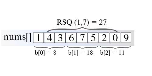
Figure 1. Range sum query using SQRT decomposition.

In the example above, the array nums's length is 9, which is split into blocks of size \sqrt{9}9​. To get RSQ(1, 7) we add b[1]. It stores the sum of range [3, 5] and partially sums from block 0 and block 2, which are overlapping boundary blocks.

Complexity Analysis

• Time complexity : O(n)O(n) - preprocessing, O(\sqrt{n})O(n​) - range sum query, O(1)O(1) - update query

  For range sum query in the worst-case scenario we have to sum approximately 3 \sqrt{n}3n​ elements. In this case the range includes \sqrt{n} - 2n​−2 blocks, which total sum costs \sqrt{n} - 2n​−2 operations. In addition to this we have to add the sum of the two boundary blocks. This takes another 2 (\sqrt{n} - 1)2(n​−1) operations. The total amount of operations is around 3 \sqrt{n}3n​.

• Space complexity : O(\sqrt{n})O(n​).

  We need additional \sqrt{n}n​ memory to store all block sums.
  
  

---

Approach 3: Segment Tree

Algorithm

Segment tree is a very flexible data structure, because it is used to solve numerous range query problems like finding minimum, maximum, sum, greatest common divisor, least common denominator in array in logarithmic time.

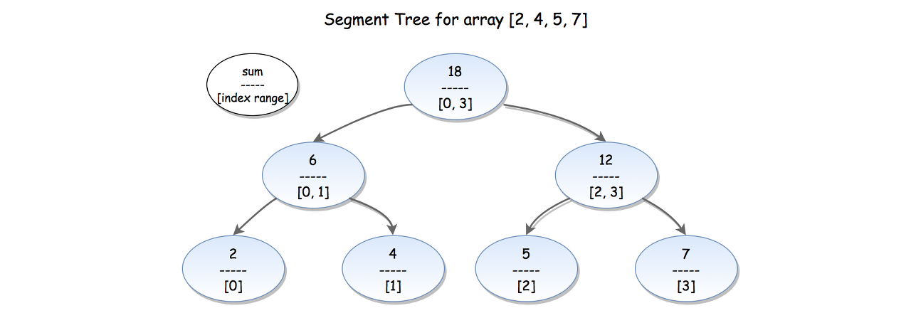
Figure 2. Illustration of Segment tree.

The segment tree for array a[0, 1, \ldots ,n-1]a[0,1,…,n−1] is a binary tree in which each node contains aggregate information (min, max, sum, etc.) for a subrange [i \ldots j][i…j] of the array, as its left and right child hold information for range [i \ldots \frac{i+j}{2}][i…2i+j​] and [\frac{i + j}{2} + 1, j][2i+j​+1,j].

Segment tree could be implemented using either an array or a tree. For an array implementation, if the element at index ii is not a leaf, its left and right child are stored at index 2i2i and 2i + 12i+1 respectively.

In the example above (Figure 2), every leaf node contains the initial array elements {2,4,5,7}. The internal nodes contain the sum of the corresponding elements in range, e.g. (6) is the sum for the elements from index 0 to index 1. The root (18) is the sum of its children (6) and (12), which also holds the total sum of the entire array.

Segment Tree can be broken down to the three following steps:

1. Pre-processing step which builds the segment tree from a given array.
2. Update the segment tree when an element is modified.
3. Calculate the Range Sum Query using the segment tree.

1. Build segment tree

We will use a very effective bottom-up approach to build segment tree. We already know from the above that if some node pp holds the sum of [i \ldots j][i…j] range, its left and right children hold the sum for range [i \ldots \frac{i + j}{2}][i…2i+j​] and [\frac{i + j}{2} + 1, j][2i+j​+1,j] respectively.

Therefore to find the sum of node pp, we need to calculate the sum of its right and left child in advance.

We begin from the leaves, initialize them with input array elements a[0, 1, \ldots, n-1]a[0,1,…,n−1]. Then we move upward to the higher level to calculate the parents' sum till we get to the root of the segment tree.

Complexity Analysis

• Time complexity : O(n)O(n)

  Time complexity is O(n)O(n), because we calculate the sum of one node during each iteration of the for loop. There are approximately 2n2n nodes in a segment tree.

  This could be proved in the following way: Segmented tree for array with nn elements has nn leaves (the array elements itself). The number of nodes in each level is half the number in the level below.

  So if we sum the number by level we will get:

  n + n/2 + n/4 + n/8 + \ldots + 1 \approx 2nn+n/2+n/4+n/8+…+1≈2n

• Space complexity : O(n)O(n).

  We used 2n2n extra space to store the segment tree.

2. Update segment tree

When we update the array at some index ii we need to rebuild the segment tree, because there are tree nodes which contain the sum of the modified element. Again we will use a bottom-up approach. We update the leaf node that stores a[i]a[i]. From there we will follow the path up to the root updating the value of each parent as a sum of its children values.

Complexity Analysis

• Time complexity : O(\log n)O(logn).

  Algorithm has O(\log n)O(logn) time complexity, because there are a few tree nodes with range that include iith array element, one on each level. There are \log(n)log(n) levels.

• Space complexity : O(1)O(1).

3. Range Sum Query

We can find range sum query [L, R][L,R] using segment tree in the following way:

Algorithm hold loop invariant:

l \le rl≤r and sum of [L \ldots l][L…l] and [r \ldots R][r…R] has been calculated, where ll and rr are the left and right boundary of calculated sum. Initially we set ll with left leaf LL and rr with right leaf RR. Range [l, r][l,r] shrinks on each iteration till range borders meets after approximately \log nlogn iterations of the algorithm

• Loop till l \le rl≤r

  • Check if ll is right child of its parent PP

    • ll is right child of PP. Then PP contains sum of range of ll and another child which is outside the range [l, r][l,r] and we don't need parent PP sum. Add ll to sumsum without its parent PP and set ll to point to the right of PP on the upper level.

    • ll is not right child of PP. Then parent PP contains sum of range which lies in [l, r][l,r]. Add PP to sumsum and set ll to point to the parent of PP

  • Check if rr is left child of its parent PP

    • rr is left child of PP. Then PP contains sum of range of rr and another child which is outside the range [l, r][l,r] and we don't need parent PP sum. Add rr to sumsum without its parent PP and set rr to point to the left of PP on the upper level.

    • rr is not left child of PP. Then parent PP contains sum of range which lies in [l, r][l,r]. Add PP to sumsum and set rr to point to the parent of PP

Complexity Analysis

• Time complexity : O(\log n)O(logn)

  Time complexity is O(\log n)O(logn) because on each iteration of the algorithm we move one level up, either to the parent of the current node or to the next sibling of parent to the left or right direction till the two boundaries meet. In the worst-case scenario this happens at the root after \log nlogn iterations of the algorithm.

• Space complexity : O(1)O(1).

Further Thoughts

The iterative version of Segment Trees was introduced in this article. A more intuitive, recursive version of Segment Trees to solve this problem is discussed here. The concept of Lazy Propagation is also introduced there.

There is an alternative solution of the problem using Binary Indexed Tree. It is faster and simpler to code. You can find it here.

 

1649 Create Sorted Array through Instructions