64. Minimum Path Sum / 741. Cherry Pickup / 1463. Cherry Pickup II

64. Minimum Path Sum

Summary

We have to find the minimum sum of numbers over a path from the top left to the bottom right of the given matrix .

Solution

Approach 1: Brute Force

The Brute Force approach involves recursion. For each element, we consider two paths, rightwards and downwards and find the minimum sum out of those two. It specifies whether we need to take a right step or downward step to minimize the sum.

\mathrm{cost}(i, j)=\mathrm{grid}[i][j] + \min \big(\mathrm{cost}(i+1, j), \mathrm{cost}(i, j+1) \big)

public class Solution {
    public int minPathSum(int[][] grid) {
        int[][] dp = new int[grid.length][grid[0].length];
        for (int i = grid.length - 1; i >= 0; i--) {
            for (int j = grid[0].length - 1; j >= 0; j--) {
                if(i == grid.length - 1 && j != grid[0].length - 1)
                    dp[i][j] = grid[i][j] +  dp[i][j + 1];
                else if(j == grid[0].length - 1 && i != grid.length - 1)
                    dp[i][j] = grid[i][j] + dp[i + 1][j];
                else if(j != grid[0].length - 1 && i != grid.length - 1)
                    dp[i][j] = grid[i][j] + Math.min(dp[i + 1][j], dp[i][j + 1]);
                else
                    dp[i][j] = grid[i][j];
            }
        }
        return dp[0][0];
    }
}

Complexity Analysis

Time complexity : O\big(2^{m+n}\big). For every move, we have atmost 2 options.
Space complexity : O(m+n). Recursion of depth m+n.

Approach 2: Dynamic Programming 2D

Algorithm

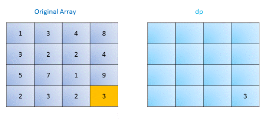
We use an extra matrix dp of the same size as the original matrix. In this matrix, dp(i, j) represents the minimum sum of the path from the index (i, j) to the bottom rightmost element. We start by initializing the bottom rightmost element of dp as the last element of the given matrix. Then for each element starting from the bottom right, we traverse backwards and fill in the matrix with the required minimum sums. Now, we need to note that at every element, we can move either rightwards or downwards. Therefore, for filling in the minimum sum, we use the equation:

dp(i, j)= \mathrm{grid}(i,j)+\min\big(dp(i+1,j),dp(i,j+1)\big)

taking care of the boundary conditions.

The following figure illustrates the process:

위에서 밑으로 가도 되고, 밑에서 위로가도 되는데, 왜 밑에서 위로 갔을까?

1 / 17

Complexity Analysis

Time complexity : O(mn). We traverse the entire matrix once.
Space complexity : O(mn). Another matrix of the same size is used.

Approach 3: Dynamic Programming 1D

Algorithm

In the previous case, instead of using a 2D matrix for dp, we can do the same work using a dp array of the row size, since for making the current entry all we need is the dp entry for the bottom and the right element. Thus, we start by initializing only the last element of the array as the last element of the given matrix. The last entry is the bottom rightmost element of the given matrix. Then, we start moving towards the left and update the entry dp(j) as:

dp(j)=\mathrm{grid}(i,j)+\min\big(dp(j),dp(j+1)\big)

We repeat the same process for every row as we move upwards. At the end dp(0) gives the required minimum sum.

Complexity Analysis

Time complexity : O(mn). We traverse the entire matrix once.
Space complexity : O(n). Another array of row size is used.

Approach 4: Dynamic Programming (Without Extra Space)

Algorithm

This approach is same as Approach 2, with a slight difference. Instead of using another dp matrix. We can store the minimum sums in the original matrix itself, since we need not retain the original matrix here. Thus, the governing equation now becomes:

\mathrm{grid}(i, j)=\mathrm{grid}(i,j)+\min \big(\mathrm{grid}(i+1,j), \mathrm{grid}(i,j+1)\big)

class Solution:
    def minPathSum(self, grid: List[List[int]]) -> int:
        m = len(grid)
        n = len(grid[0])
        
        for i in range(m):
            for j in range(n):
                if i-1 >= 0 and j-1 >= 0:
                    grid[i][j] += min(grid[i-1][j], grid[i][j-1])
                elif i-1 >= 0:
                    grid[i][j] += grid[i-1][j]
                elif j-1 >= 0:
                    grid[i][j] += grid[i][j-1]
        
        return grid[m-1][n-1]

Complexity Analysis

Time complexity : O(mn). We traverse the entire matrix once.
Space complexity : O(1). No extra space is used.

741. Cherry Pickup

leetcode.com/problems/cherry-pickup/

Cherry Pickup - LeetCode

Level up your coding skills and quickly land a job. This is the best place to expand your knowledge and get prepared for your next interview.

leetcode.com

You are given an n x n grid representing a field of cherries, each cell is one of three possible integers.

0 means the cell is empty, so you can pass through,
1 means the cell contains a cherry that you can pick up and pass through, or
-1 means the cell contains a thorn that blocks your way.

Return the maximum number of cherries you can collect by following the rules below:

Starting at the position (0, 0) and reaching (n - 1, n - 1) by moving right or down through valid path cells (cells with value 0 or 1).
After reaching (n - 1, n - 1), returning to (0, 0) by moving left or up through valid path cells.
When passing through a path cell containing a cherry, you pick it up, and the cell becomes an empty cell 0.
If there is no valid path between (0, 0) and (n - 1, n - 1), then no cherries can be collected.

Example 1:

Input: grid = [[0,1,-1],[1,0,-1],[1,1,1]] Output: 5 Explanation: The player started at (0, 0) and went down, down, right right to reach (2, 2). 4 cherries were picked up during this single trip, and the matrix becomes [[0,1,-1],[0,0,-1],[0,0,0]]. Then, the player went left, up, up, left to return home, picking up one more cherry. The total number of cherries picked up is 5, and this is the maximum possible.

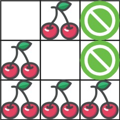
Example 2:

Input: grid = [[1,1,-1],[1,-1,1],[-1,1,1]] Output: 0

Constraints:

n == grid.length
n == grid[i].length
1 <= n <= 50
grid[i][j] is -1, 0, or 1.
grid[0][0] != -1
grid[n - 1][n - 1] != -1

Approach #1: Greedy [Wrong Answer]

Intuition

Let's find the most cherries we can pick up with one path, pick them up, then find the most cherries we can pick up with a second path on the remaining field.

Though a counter example might be hard to think of, this approach fails to find the best answer to this case:

11100 00101 10100 00100 00111

Algorithm

We can use dynamic programming to find the most number of cherries dp[i][j] that can be picked up from any location (i, j) to the bottom right corner. This is a classic question very similar to Minimum Path Sum, refer to the link if you are not familiar with this type of question.

After, we can find an first path that maximizes the number of cherries taken by using our completed dp as an oracle for deciding where to move. We'll choose the move that allows us to pick up more cherries (based on comparing dp[i+1][j] and dp[i][j+1]).

After taking the cherries from that path (and removing it from the grid), we'll take the cherries again.

Complexity Analysis

Time Complexity: O(N^2), where N is the length of grid. Our dynamic programming consists of two for-loops of length N.
Space Complexity: O(N^2), the size of dp.

Approach #2: Dynamic Programming (Top Down) [Accepted]

Intuition

Instead of walking from end to beginning, let's reverse the second leg of the path, so we are only considering two paths from the beginning to the end.

Notice after t steps, each position (r, c) we could be, is on the line r + c = t. So if we have two people at positions (r1, c1) and (r2, c2), then r2 = r1 + c1 - c2. That means the variables r1, c1, c2 uniquely determine 2 people who have walked the same r1 + c1 number of steps. This sets us up for dynamic programming quite nicely.

Algorithm

Let dp[r1][c1][c2] be the most number of cherries obtained by two people starting at (r1, c1) and (r2, c2) and walking towards (N-1, N-1) picking up cherries, where r2 = r1+c1-c2.

If grid[r1][c1] and grid[r2][c2] are not thorns, then the value of dp[r1][c1][c2] is (grid[r1][c1] + grid[r2][c2]), plus the maximum of dp[r1+1][c1][c2], dp[r1][c1+1][c2], dp[r1+1][c1][c2+1], dp[r1][c1+1][c2+1] as appropriate. We should also be careful to not double count in case (r1, c1) == (r2, c2).

Why did we say it was the maximum of dp[r+1][c1][c2] etc.? It corresponds to the 4 possibilities for person 1 and 2 moving down and right:

Person 1 down and person 2 down: dp[r1+1][c1][c2];
Person 1 right and person 2 down: dp[r1][c1+1][c2];
Person 1 down and person 2 right: dp[r1+1][c1][c2+1];
Person 1 right and person 2 right: dp[r1][c1+1][c2+1];

class Solution:
    def cherryPickup(self, grid: List[List[int]]) -> int:
        # after t steps, (r,c) => r + c = t
        # for 2 people : r1+c1 = r2 + c2 => r2 = r1 + c1 - c2
        N = len(grid)
        memo = [[[None] * N for _1 in range(N)] for _2 in range(N)]
        def dp(r1, c1, c2):
            r2 = r1 + c1 - c2
            if(N==r1 or N==r2 or N==c1 or N==c2 or grid[r1][c1] == -1 or grid[r2][c2] == -1):
                return float('-inf')
            elif r1 == c1 == N-1:
                return grid[r1][c1]
            elif memo[r1][c1][c2] is not None:
                return memo[r1][c1][c2]
            else:
                ans = grid[r1][c1] + (c1 != c2) * grid[r2][c2]
                ans += max(dp(r1, c1+1, c2+1), dp(r1+1, c1, c2+1), dp(r1, c1+1, c2), dp(r1+1, c1, c2))
            memo[r1][c1][c2] = ans
            return ans
        return max(0, dp(0,0,0))

Complexity Analysis

Time Complexity: O(N^3), where N is the length of grid. Our dynamic programming has O(N^3) states.
Space Complexity: O(N^3), the size of memo.

Approach #3: Dynamic Programming (Bottom Up) [Accepted]

Intuition

Like in Approach #2, we have the idea of dynamic programming.

Say r1 + c1 = t is the t-th layer. Since our recursion only references the next layer, we only need to keep two layers in memory at a time.

Algorithm

At time t, let dp[c1][c2] be the most cherries that we can pick up for two people going from (0, 0) to (r1, c1) and (0, 0) to (r2, c2), where r1 = t-c1, r2 = t-c2. Our dynamic program proceeds similarly to Approach #2.

class Solution:
    def cherryPickup(self, grid: List[List[int]]) -> int:
        N = len(grid)
        dp = [[float('-inf')] * N for _ in range(N)]
        dp[0][0] = grid[0][0]
        for t in range(1, 2*N-1):
            dp2 = [[float('-inf')]*N for _ in range(N)]
            for i in range(max(0, t-(N-1)), min(N-1, t) + 1):
                for j in range(max(0, t-(N-1)), min(N-1, t) + 1):
                    if grid[i][t-i] == -1 or grid[j][t-j] == -1:
                        continue
                    val = grid[i][t-i]
                    if i != j: val += grid[j][t-j]
                    dp2[i][j] = max(dp[pi][pj] + val
                            for pi in (i-1, i) for pj in (j-1, j)
                                if pi >= 0 and pj >= 0)
            dp = dp2
        return max(0, dp[N-1][N-1])

Complexity Analysis

Time Complexity: O(N^3), where N is the length of grid. We have three for-loops of size O(N).
Space Complexity: O(N^2), the sizes of dp and dp2.

ㅡㅡ;;;;;

leetcode.com/problems/dungeon-game/

leetcode.com/problems/unique-paths/

1463. Cherry Pickup II

Given a rows x cols matrix grid representing a field of cherries. Each cell in grid represents the number of cherries that you can collect.

You have two robots that can collect cherries for you, Robot #1 is located at the top-left corner (0,0) , and Robot #2 is located at the top-right corner (0, cols-1) of the grid.

Return the maximum number of cherries collection using both robots by following the rules below:

From a cell (i,j), robots can move to cell (i+1, j-1) , (i+1, j) or (i+1, j+1).
When any robot is passing through a cell, It picks it up all cherries, and the cell becomes an empty cell (0).
When both robots stay on the same cell, only one of them takes the cherries.
Both robots cannot move outside of the grid at any moment.
Both robots should reach the bottom row in the grid.

Example 1:

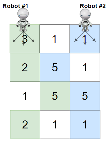
Input: grid = [[3,1,1],[2,5,1],[1,5,5],[2,1,1]] Output: 24 Explanation: Path of robot #1 and #2 are described in color green and blue respectively. Cherries taken by Robot #1, (3 + 2 + 5 + 2) = 12. Cherries taken by Robot #2, (1 + 5 + 5 + 1) = 12. Total of cherries: 12 + 12 = 24.

Example 2:

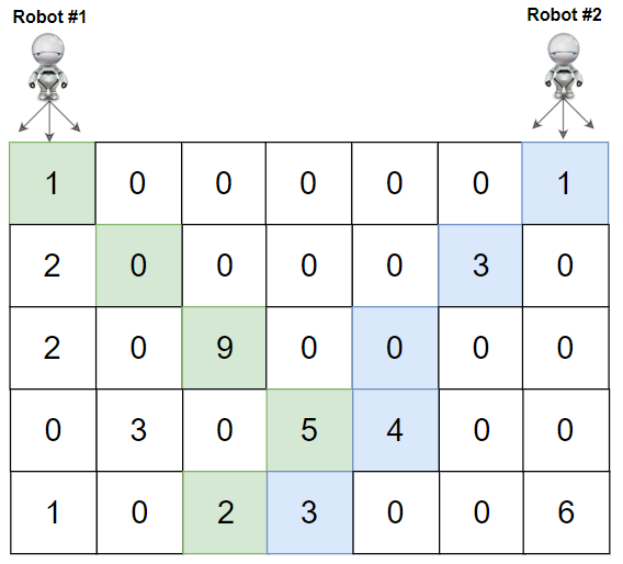
Input: grid = [[1,0,0,0,0,0,1],[2,0,0,0,0,3,0],[2,0,9,0,0,0,0],[0,3,0,5,4,0,0],[1,0,2,3,0,0,6]] Output: 28 Explanation: Path of robot #1 and #2 are described in color green and blue respectively. Cherries taken by Robot #1, (1 + 9 + 5 + 2) = 17. Cherries taken by Robot #2, (1 + 3 + 4 + 3) = 11. Total of cherries: 17 + 11 = 28.

Example 3:

Input: grid = [[1,0,0,3],[0,0,0,3],[0,0,3,3],[9,0,3,3]] Output: 22

Example 4:

Input: grid = [[1,1],[1,1]] Output: 4

Constraints:

rows == grid.length
cols == grid[i].length
2 <= rows, cols <= 70
0 <= grid[i][j] <= 100

Use dynammic programming, define DP[i][j][k]: The maximum cherries that both robots can take starting on the ith row, and column j and k of Robot 1 and 2 respectively.

Overview

You probably can guess from the problem title that this problem is an extension of the original Cherry Pickup.

In this problem, we do not need to return to the starting point but have two robots instead of one. However, the essence of this problem does not change, and the same method is still available.

Below, we will discuss two similar approaches: Dynamic Programming (Top Down) and Dynamic Programming (Bottom Up).

The first one is also known as dfs with memoization or memoization dp, and the second one is also known as tabulation dp. They have the same main idea but different coding approaches.

Approach #1: Dynamic Programming (Top Down)

Intuition

In this part, we will explain how to think of this approach step by step.

If you are only interested in the pure algorithm, you can jump to the algorithm part.

We need to move two robots! Note that the order of moving robot1 or robot2 does not matter since it would not impact the cherries we can pick. The number of cherries we can pick only depends on the tracks of our robots.

Therefore, we can move the robot1 and robot2 in any order we want. We aim to apply DP, so we are looking for an order that suitable for DP.

Let's try a few possible moving orders.

Can we move robot1 firstly to the bottom row, and then move robot2?

Maybe not. In this case, the movement of robot1 will impact the movement of robot2. In other words, the optimal track of robot2 depends on the track of robot1. If we want to apply DP, we need to record the whole track of robot1 as the state. The number of sub-problems is too much.

In fact, in any case, when we move one robot several steps earlier than the other, the movement of the first robot will impact the movement of the second robot.

Unless we move them synchronously (i.e., move one step of robot1 and robot2 at the same time).

Let's define the DP state as (row1, col1, row2, col2), where (row1, col1) represents the location of robot1, and (row2, col2) represents the location of robot2.

If we move them synchronously, robot1 and robot2 will always on the same row. Therefore, row1 == row2.

Let row = row1. The DP state is simplified to (row, col1, col2), where (row, col1) represents the location of robot1, and (row, col2) represents the location of robot2.

OK, time to define the DP function.

Since it's a top-down DP approach, we try to solve the problem with the DP function. Check approach 2 for DP array (bottom-up).

Let dp(row, col1, col2) return the maximum cherries we can pick if robot1 starts at (row, col1) and robot2 starts at (row, col2).

You can try changing different dp meaning to yield some other similar approaches. For example, let dp(row, col1, col2) mean the maximum cherries we can pick if robot1 ends at (row, col1) and robot2 ends at (row, col2).

The base cases are that robot1 and robot2 both start at the bottom line. In this case, they do not need to move. All we need to do is to collect the cherries at current cells. Remember not to double count if robot1 and robot2 are at exactly the same cell.

In other cases, we need to add the maximum cherries robots can pick in the future. Here comes the transition function.

Since we move robots synchronously, and each robot has three different movements for one step, we totally have 3*3 = 9 possible movements for two robots:

The maximum cherries robots can pick in the future would be the max of those 9 movements, which is the maximum of dp(row+1, new_col1, new_col2), where new_col1 can be col1, col1+1, or col1-1, and new_col2 can be col2, col2+1, or col2-1.

Remember to use a map or an array to store the results of our dp function to prevent redundant calculating.

Algorithm

Define a dp function that takes three integers row, col1, and col2 as input.

(row, col1) represents the location of robot1, and (row, col2) represents the location of robot2.

The dp function returns the maximum cherries we can pick if robot1 starts at (row, col1) and robot2 starts at (row, col2).

In the dp function:

Collect the cherry at (row, col1) and (row, col2). Do not double count if col1 == col2.
If we do not reach the last row, we need to add the maximum cherries we can pick in the future.
The maximum cherries we can pick in the future is the maximum of dp(row+1, new_col1, new_col2), where new_col1 can be col1, col1+1, or col1-1, and new_col2 can be col2, col2+1, or col2-1.
Return the total cherries we can pick.

Finally, return dp(row=0, col1=0, col2=last_column) in the main function.

Implementation

class Solution:
    def cherryPickup(self, grid: List[List[int]]) -> int:
        m = len(grid)
        n = len(grid[0])

        @lru_cache(None)
        def dp(row, col1, col2):
            if col1 < 0 or col1 >= n or col2 < 0 or col2 >= n:
                return -inf
            # current cell
            result = 0
            result += grid[row][col1]
            if col1 != col2:
                result += grid[row][col2]
            # transition
            if row != m-1:
                result += max(dp(row+1, new_col1, new_col2)
                              for new_col1 in [col1, col1+1, col1-1]
                              for new_col2 in [col2, col2+1, col2-1])
            return result

        return dp(0, 0, n-1)

Complexity Analysis

Let M be the number of rows in grid and N be the number of columns in grid.

Time Complexity: \mathcal{O}(MN^2), since our helper function have three variables as input, which have M, N, and N possible values respectively. In the worst case, we have to calculate them all once, so that would cost \mathcal{O}(M \cdot N \cdot N) = \mathcal{O}(MN^2). Also, since we save the results after calculating, we would not have repeated calculation.
Space Complexity: \mathcal{O}(MN^2), since our helper function have three variables as input, and they have M, N, and N possible values respectively. We need a map with size of \mathcal{O}(M \cdot N \cdot N) = \mathcal{O}(MN^2) to store the results.

Approach #2: Dynamic Programming (Bottom Up)

Intuition

Similarly, we need a three-dimension array dp[row][col1][col2] to store calculated results:

dp[row][col1][col2] represents the maximum cherries we can pick if robot1 starts at (row, col1) and robot2 starts at (row, col2).

Remember, we move robot1 and robot2 synchronously, so they are always on the same row.

The base cases are that robot1 and robot2 both start at the bottom row. In this case, we only need to calculate the cherry at current cells.

Otherwise, apply the transition equation to get the maximum cherries we can pick in the future.

Since the base case is at the bottom row, we need to iterate from the bottom row to the top row when filling the dp array.

You can use state compression to save the first dimension since we only need dp[row+1] when calculating dp[row].

You can change the meaning of dp[row][col1][col2] and some corresponding codes to get some other similar approaches. For example, let dp[row][col1][col2] mean the maximum cherries we can pick if robot1 ends at (row, col1) and robot2 ends at (row, col2).

Algorithm

Define a three-dimension dp array where each dimension has a size of m, n, and n respectively.

dp[row][col1][col2] represents the maximum cherries we can pick if robot1 starts at (row, col1) and robot2 starts at (row, col2).

To compute dp[row][col1][col2] (transition equation):

Collect the cherry at (row, col1) and (row, col2). Do not double count if col1 == col2.
If we are not in the last row, we need to add the maximum cherries we can pick in the future.
The maximum cherries we can pick in the future is the maximum of dp[row+1][new_col1][new_col2], where new_col1 can be col1, col1+1, or col1-1, and new_col2 can be col2, col2+1, or col2-1.

Finally, return dp[0][0][last_column].

State compression can be used to save the first dimension: dp[col1][col2]. Just reuse the dp array after iterating one row.

Implementation

class Solution:
    def cherryPickup(self, grid: List[List[int]]) -> int:
        m = len(grid)
        n = len(grid[0])
        dp = [[[0]*n for _ in range(n)] for __ in range(m)]

        for row in reversed(range(m)):
            for col1 in range(n):
                for col2 in range(n):
                    result = 0
                    # current cell
                    result += grid[row][col1]
                    if col1 != col2:
                        result += grid[row][col2]
                    # transition
                    if row != m-1:
                        result += max(dp[row+1][new_col1][new_col2]
                                      for new_col1 in [col1, col1+1, col1-1]
                                      for new_col2 in [col2, col2+1, col2-1]
                                      if 0 <= new_col1 < n and 0 <= new_col2 < n)
                    dp[row][col1][col2] = result
        return dp[0][0][n-1]

Complexity Analysis

Let M be the number of rows in grid and N be the number of columns in grid.

Time Complexity: \mathcal{O}(MN^2), since our dynamic programming has three nested for-loops, which have M, N, and N iterations respectively. In total, it costs \mathcal{O}(M \cdot N \cdot N) = \mathcal{O}(MN^2).
Space Complexity: \mathcal{O}(MN^2) if not use state compression, since our dp array has \mathcal{O}(M \cdot N \cdot N) = \mathcal{O}(MN^2) elements. \mathcal{O}(N^2) if use state compression, since we can reuse the first dimension, and our dp array only has \mathcal{O}(N \cdot N) = \mathcal{O}(N^2) elements.