Trees and Graphs - Top Interview Questions[Medium] (3/9) : Python
Trees and Graphs
트리는 특별한 유형의 그래프이므로 그래프를 가로 지르는 데 사용되는 두 가지 일반적인 기술도 트리에 적용 할 수 있습니다.
권장 사항 : 이진 트리 순서 순회, 각 노드 및 아일랜드 수에서 다음 오른쪽 포인터 채우기.
일부 트리 문제는 n 진 트리 형식으로도 질문 할 수 있으므로 n 진 트리가 무엇인지 알아야합니다.
참고 : Number of Islands는 트리 문제는 아니지만 그래프로 표시 할 수 있으므로 그래프 문제로 분류합니다.
Tree is a special type of graphs, so the two usual techniques used to traverse a graph are also applicable to trees.
We recommend: Binary Tree Inorder Traversal, Populating Next Right Pointers in Each Node and Number of Islands.
Note that some of the tree problems can also be asked in n-ary tree format, so make sure you know what an n-ary tree is.
Note: Although Number of Islands is not a tree problem, it can be represented as a graph and therefore we categorize it as a graph problem.
Binary Tree Inorder Traversal
Binary Tree Zigzag Level Order Traversal
Construct Binary Tree from Preorder and Inorder Traversal
Populating Next Right Pointers in Each Node
Kth Smallest Element in a BST
Inorder Successor in BST
Number of Islands
94. Binary Tree Inorder Traversal
leetcode.com/problems/binary-tree-inorder-traversal/solution/
Medium
4075177Add to ListShare
Given the root of a binary tree, return the inorder traversal of its nodes' values.
Example 1:
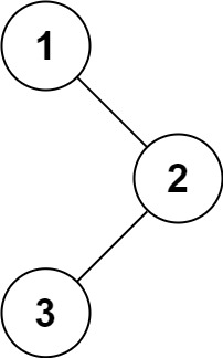
Input: root = [1,null,2,3] Output: [1,3,2]
Example 2:
Input: root = [] Output: []
Example 3:
Input: root = [1] Output: [1]
Example 4:
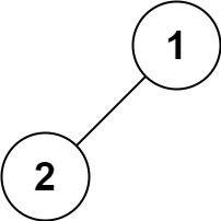
Input: root = [1,2] Output: [2,1]
Example 5:
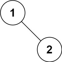
Input: root = [1,null,2] Output: [1,2]
Constraints:
- The number of nodes in the tree is in the range [0, 100].
- -100 <= Node.val <= 100
Follow up:
Recursive solution is trivial, could you do it iteratively?
Approach 1: Recursive Approach
The first method to solve this problem is using recursion. This is the classical method and is straightforward. We can define a helper function to implement recursion.
class Solution:
    def inorderTraversal(self, root: TreeNode) -> List[int]:
        ans = []
        def inorder(node:TreeNode):
            if not node:
                return
            inorder(node.left)
            ans.append(node.val)
            inorder(node.right)

        inorder(root)

        return ans
Complexity Analysis
-
Time complexity : O(n)O(n). The time complexity is O(n)O(n) because the recursive function is T(n) = 2 \cdot T(n/2)+1T(n)=2⋅T(n/2)+1.
-
Space complexity : The worst case space required is O(n)O(n), and in the average case it's O(\log n)O(logn) where nn is number of nodes.
Approach 2: Iterating method using Stack
The strategy is very similiar to the first method, the different is using stack.
Here is an illustration:
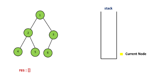
1 / 14
Complexity Analysis
-
Time complexity : O(n)O(n).
-
Space complexity : O(n)O(n).
Approach 3: Morris Traversal
In this method, we have to use a new data structure-Threaded Binary Tree, and the strategy is as follows:
Step 1: Initialize current as root
Step 2: While current is not NULL,
If current does not have left child a. Add current’s value b. Go to the right, i.e., current = current.right Else a. In current's left subtree, make current the right child of the rightmost node b. Go to this left child, i.e., current = current.left
For example:
1 / \ 2 3 / \ / 4 5 6
First, 1 is the root, so initialize 1 as current, 1 has left child which is 2, the current's left subtree is
2 / \ 4 5
So in this subtree, the rightmost node is 5, then make the current(1) as the right child of 5. Set current = cuurent.left (current = 2). The tree now looks like:
2 / \ 4 5 \ 1 \ 3 / 6
For current 2, which has left child 4, we can continue with thesame process as we did above
4 \ 2 \ 5 \ 1 \ 3 / 6
then add 4 because it has no left child, then add 2, 5, 1, 3 one by one, for node 3 which has left child 6, do the same as above. Finally, the inorder taversal is [4,2,5,1,6,3].
For more details, please check Threaded binary tree and Explaination of Morris Method
Complexity Analysis
-
Time complexity : O(n)O(n). To prove that the time complexity is O(n)O(n), the biggest problem lies in finding the time complexity of finding the predecessor nodes of all the nodes in the binary tree. Intuitively, the complexity is O(n\log n)O(nlogn), because to find the predecessor node for a single node related to the height of the tree. But in fact, finding the predecessor nodes for all nodes only needs O(n)O(n) time. Because a binary Tree with nn nodes has n-1n−1 edges, the whole processing for each edges up to 2 times, one is to locate a node, and the other is to find the predecessor node. So the complexity is O(n)O(n).
-
Space complexity : O(n)O(n). Arraylist of size nn is used.
leetcode.com/problems/binary-tree-zigzag-level-order-traversal/solution/
103. Binary Tree Zigzag Level Order Traversal
Medium
2918118Add to ListShare
Given a binary tree, return the zigzag level order traversal of its nodes' values. (ie, from left to right, then right to left for the next level and alternate between).
For example:
Given binary tree [3,9,20,null,null,15,7],
3 / \ 9 20 / \ 15 7
return its zigzag level order traversal as:
[ [3], [20,9], [15,7] ]
Solution
Approach 1: BFS (Breadth-First Search)
Intuition
Following the description of the problem, the most intuitive solution would be the BFS (Breadth-First Search) approach through which we traverse the tree level-by-level.
The default ordering of BFS within a single level is from left to right. As a result, we should adjust the BFS algorithm a bit to generate the desired zigzag ordering.
One of the keys here is to store the values that are of the same level with the deque (double-ended queue) data structure, where we could add new values on either end of a queue.
So if we want to have the ordering of FIFO (first-in-first-out), we simply append the new elements to the tail of the queue, i.e. the late comers stand last in the queue. While if we want to have the ordering of FILO (first-in-last-out), we insert the new elements to the head of the queue, i.e. the late comers jump the queue.
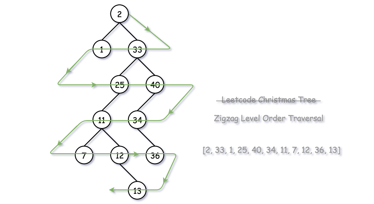
Algorithm
There are several ways to implement the BFS algorithm.
- One way would be that we run a two-level nested loop, with the outer loop iterating each level on the tree, and with the inner loop iterating each node within a single level.
- We could also implement BFS with a single loop though. The trick is that we append the nodes to be visited into a queue and we separate nodes of different levels with a sort of delimiter (e.g. an empty node). The delimiter marks the end of a level, as well as the beginning of a new level.
Here we adopt the second approach above. One can start with the normal BFS algorithm, upon which we add a touch of zigzag order with the help of deque. For each level, we start from an empty deque container to hold all the values of the same level. Depending on the ordering of each level, i.e. either from-left-to-right or from-right-to-left, we decide at which end of the deque to add the new element:

-
For the ordering of from-left-to-right (FIFO), we append the new element to the tail of the queue, so that the element that comes late would get out late as well. As we can see from the above graph, given an input sequence of [1, 2, 3, 4, 5], with FIFO ordering, we would have an output sequence of [1, 2, 3, 4, 5].
-
For the ordering of from-right-to-left (FILO), we insert the new element to the head of the queue, so that the element that comes late would get out first. With the same input sequence of [1, 2, 3, 4, 5], with FILO ordering, we would obtain an output sequence of [5, 4, 3, 2, 1].
Note: as an alternative approach, one can also implement the normal BFS algorithm first, which would generate the ordering of from-left-to-right for each of the levels. Then, at the end of the algorithm, we can simply reverse the ordering of certain levels, following the zigzag steps.
Complexity Analysis
-
Time Complexity: \mathcal{O}(N)O(N), where NN is the number of nodes in the tree.
-
We visit each node once and only once.
-
In addition, the insertion operation on either end of the deque takes a constant time, rather than using the array/list data structure where the inserting at the head could take the \mathcal{O}(K)O(K) time where KK is the length of the list.
-
-
Space Complexity: \mathcal{O}(N)O(N) where NN is the number of nodes in the tree.
-
The main memory consumption of the algorithm is the node_queue that we use for the loop, apart from the array that we use to keep the final output.
-
As one can see, at any given moment, the node_queue would hold the nodes that are at most across two levels. Therefore, at most, the size of the queue would be no more than 2 \cdot L2⋅L, assuming LL is the maximum number of nodes that might reside on the same level. Since we have a binary tree, the level that contains the most nodes could occur to consist all the leave nodes in a full binary tree, which is roughly L = \frac{N}{2}L=2N. As a result, we have the space complexity of 2 \cdot \frac{N}{2} = N2⋅2N=N in the worst case.
-
Approach 2: DFS (Depth-First Search)
Intuition
Though not intuitive, we could also obtain the BFS traversal ordering via the DFS (Depth-First Search) traversal in the tree.
The trick is that during the DFS traversal, we maintain the results in a global array that is indexed by the level, i.e. the element array[level] would contain all the nodes that are at the same level. The global array would then be referred and updated at each step of DFS.
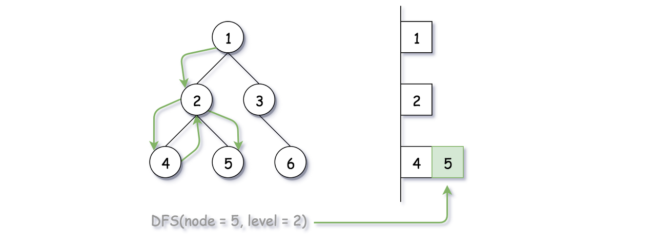
Similar with the above modified BFS algorithm, we employ the deque data structure to hold the nodes that are of the same level, and we alternate the insertion direction (i.e. either to the head or to the tail) to generate the desired output ordering.
Algorithm
Here we implement the DFS algorithm via recursion. We define a recursive function called DFS(node, level) which only takes care of the current node which is located at the specified level. Within the function, here are three steps that we would perform:
-
If this is the first time that we visit any node at the level, i.e. the deque for the level does not exist, then we simply create the deque with the current node value as the initial element.
-
If the deque for this level exists, then depending on the ordering, we insert the current node value either to the head or to the tail of the queue.
-
At the end, we recursively call the function for each of its child nodes.
It might go without saying that, one can also implement the DFS traversal via iteration rather than recursion, which could be one of the followup questions by an interviewer.
Complexity Analysis
-
Time Complexity: \mathcal{O}(N)O(N), where NN is the number of nodes in the tree.
- Same as the previous BFS approach, we visit each node once and only once.
-
Space Complexity: \mathcal{O}(H)O(H), where HH is the height of the tree, i.e. the number of levels in the tree, which would be roughly \log_2{N}log2N.
-
Unlike the BFS approach, in the DFS approach, we do not need to maintain the node_queue data structure for the traversal.
-
However, the function recursion would incur additional memory consumption on the function call stack. As we can see, the size of the call stack for any invocation of DFS(node, level) would be exactly the number of level that the current node resides on. Therefore, the space complexity of our DFS algorithm is \mathcal{O}(\log_2{N})O(log2N) which is much better than the BFS approach.
-
leetcode.com/problems/construct-binary-tree-from-preorder-and-inorder-traversal/solution/
leetcode.com/problems/populating-next-right-pointers-in-each-node/solution/
leetcode.com/problems/kth-smallest-element-in-a-bst/solution/
leetcode.com/problems/inorder-successor-in-bst/solution/
200. Number of Islands
leetcode.com/problems/number-of-islands/solution/
Medium
7315229Add to ListShare
Given an m x n 2d grid map of '1's (land) and '0's (water), return the number of islands.
An island is surrounded by water and is formed by connecting adjacent lands horizontally or vertically. You may assume all four edges of the grid are all surrounded by water.
Example 1:
Input: grid = [ ["1","1","1","1","0"], ["1","1","0","1","0"], ["1","1","0","0","0"], ["0","0","0","0","0"] ] Output: 1
Example 2:
Input: grid = [ ["1","1","0","0","0"], ["1","1","0","0","0"], ["0","0","1","0","0"], ["0","0","0","1","1"] ] Output: 3
Constraints:
- m == grid.length
- n == grid[i].length
- 1 <= m, n <= 300
- grid[i][j] is '0' or '1'.
Approach #1 DFS [Accepted]
Intuition
Treat the 2d grid map as an undirected graph and there is an edge between two horizontally or vertically adjacent nodes of value '1'.
Algorithm
Linear scan the 2d grid map, if a node contains a '1', then it is a root node that triggers a Depth First Search. During DFS, every visited node should be set as '0' to mark as visited node. Count the number of root nodes that trigger DFS, this number would be the number of islands since each DFS starting at some root identifies an island.
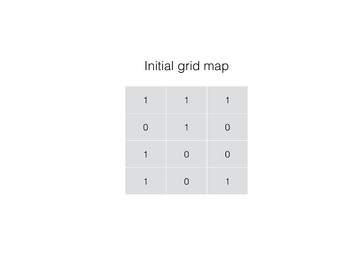
1 / 8
class Solution:
    def numIslands(self, grid: List[List[str]]) -> int:
        cnt = 0
        r = len(grid)
        c = len(grid[0])
        print(r, c)

        def go(i:int, j:int, grid: List[List[str]]):
            if 0 <= i < r and 0 <= j < c:
                if grid[i][j] == '1':
                    grid[i][j] = '0'
                    go(i+1, j, grid)
                    go(i, j+1, grid)
                    go(i-1, j, grid)
                    go(i, j-1, grid)

        for i in range(r):
            for j in range(c):
                if grid[i][j] == '1':
                    cnt += 1
                    go(i, j, grid)

        return cnt
Complexity Analysis
-
Time complexity : O(M \times N)O(M×N) where MM is the number of rows and NN is the number of columns.
-
Space complexity : worst case O(M \times N)O(M×N) in case that the grid map is filled with lands where DFS goes by M \times NM×N deep.
Approach #2: BFS [Accepted]
Algorithm
Linear scan the 2d grid map, if a node contains a '1', then it is a root node that triggers a Breadth First Search. Put it into a queue and set its value as '0' to mark as visited node. Iteratively search the neighbors of enqueued nodes until the queue becomes empty.
class Solution:
    def numIslands(self, grid: List[List[str]]) -> int:
        r = len(grid)
        if r == 0: return 0
        c = len(grid[0])

        cnt = 0

        for i in range(r):
            for j in range(c):
                if grid[i][j] == '1':
                    cnt += 1

                    que = deque()
                    que.append((i, j))

                    while que:
                        a, b = que.popleft()
                        if 0 <= a < r and 0 <= b < c:
                            grid[a][b] = '0'
                            que.append((a-1, b))
                            que.append((a, b-1))
                            que.append((a+1, b))
                            que.append((a, b+1))

        return cnt
Complexity Analysis
-
Time complexity : O(M \times N)O(M×N) where MM is the number of rows and NN is the number of columns.
-
Space complexity : O(min(M, N))O(min(M,N)) because in worst case where the grid is filled with lands, the size of queue can grow up to min(M,NM,N).
Approach #3: Union Find (aka Disjoint Set) [Accepted]
Algorithm
Traverse the 2d grid map and union adjacent lands horizontally or vertically, at the end, return the number of connected components maintained in the UnionFind data structure.
For details regarding to Union Find, you can refer to this article.

python union find code
www.geeksforgeeks.org/union-find/
from collections import defaultdict

#This class represents a undirected graph using adjacency list representation
class Graph:

    def __init__(self,vertices):
        self.V= vertices #No. of vertices
        self.graph = defaultdict(list) # default dictionary to store graph


    # function to add an edge to graph
    def addEdge(self,u,v):
        self.graph[u].append(v)

    # A utility function to find the subset of an element i
    def find_parent(self, parent,i):
        if parent[i] == -1:
            return i
        if parent[i]!= -1:
             return self.find_parent(parent,parent[i])

    # A utility function to do union of two subsets
    def union(self,parent,x,y):
        x_set = self.find_parent(parent, x)
        y_set = self.find_parent(parent, y)
        parent[x_set] = y_set


    # The main function to check whether a given graph
    # contains cycle or not
    def isCyclic(self):

        # Allocate memory for creating V subsets and
        # Initialize all subsets as single element sets
        parent = [-1]*(self.V)

        # Iterate through all edges of graph, find subset of both
        # vertices of every edge, if both subsets are same, then
        # there is cycle in graph.
        for i in self.graph:
            for j in self.graph[i]:
                x = self.find_parent(parent, i)
                y = self.find_parent(parent, j)
                if x == y:
                    return True
                self.union(parent,x,y)


# Create a graph given in the above diagram
g = Graph(3)
g.addEdge(0, 1)
g.addEdge(1, 2)
g.addEdge(2, 0)

if g.isCyclic():
    print "Graph contains cycle"
else :
    print "Graph does not contain cycle "
1 / 6
Complexity Analysis
-
Time complexity : O(M \times N)O(M×N) where MM is the number of rows and NN is the number of columns. Note that Union operation takes essentially constant time[1] when UnionFind is implemented with both path compression and union by rank.
-
Space complexity : O(M \times N)O(M×N) as required by UnionFind data structure.
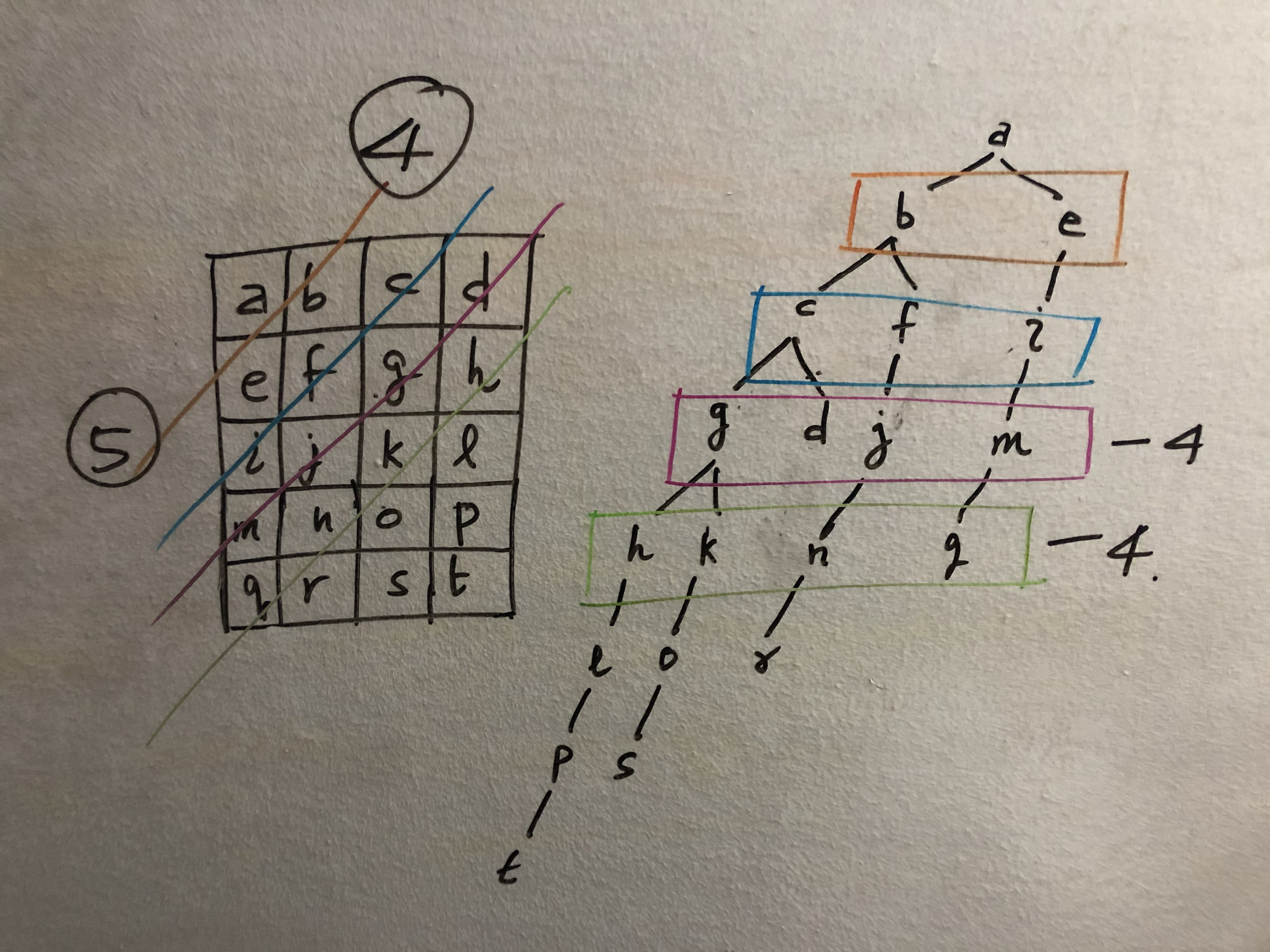
위의 문제에 추가문제.
'[영문사이트] LeetCode 리트코드/[Medium]Top Interview Questions' 의 관련글
-
Sorting and Searching - Top Interview Questions[Medium] (5/9) : Python 2020.12.22더보기
-
Backtracking - Top Interview Questions[Medium] (4/9) : Python 2020.12.22더보기
-
Linked List - Top Interview Questions[Medium] (2/9) : Python 2020.12.22더보기
-
Array and Strings - Top Interview Questions[Medium] (1/9) : Python 2020.12.22더보기


